Steps to use a ML model in TensorflowJS

TensorFlow.js — Making Predictions from 2D Data  |  Google Codelabs

1: Create the model

Creates a sequential model with a Dense Layer.

function createModel() {
  // Create a sequential model
  const model = tf.sequential();
 
  // Add a single input layer
  model.add(tf.layers.dense({inputShape: [1], units: 1, useBias: true}));
 
  // Add an output layer
  model.add(tf.layers.dense({units: 1, useBias: true}));
 
  return model;
}

Add layers

This adds an input layer to the network. That input layer is connected to a dense layer.

model.add(tf.layers.dense({inputShape: [1], units: 1, useBias: true}));

You also define the inputShape.

Then define the output layer. units is 1 because it should output 1 number.

model.add(tf.layers.dense({units: 1}));

2: Prepare the data

It is best practice to perform shuffling and normalisation on training data.

Data needs to be converted to tensors to make training models practical.

/**
 * Convert the input data to tensors that we can use for machine
 * learning. We will also do the important best practices of _shuffling_
 * the data and _normalizing_ the data
 * MPG on the y-axis.
 */
function convertToTensor(data) {
  // Wrapping these calculations in a tidy will dispose any
  // intermediate tensors.
 
  return tf.tidy(() => {
    // Step 1. Shuffle the data
    tf.util.shuffle(data);
 
    // Step 2. Convert data to Tensor
    const inputs = data.map(d => d.horsepower)
    const labels = data.map(d => d.mpg);
 
    const inputTensor = tf.tensor2d(inputs, [inputs.length, 1]);
    const labelTensor = tf.tensor2d(labels, [labels.length, 1]);
 
    //Step 3. Normalize the data to the range 0 - 1 using min-max scaling
    const inputMax = inputTensor.max();
    const inputMin = inputTensor.min();
    const labelMax = labelTensor.max();
    const labelMin = labelTensor.min();
 
    const normalizedInputs = inputTensor.sub(inputMin).div(inputMax.sub(inputMin));
    const normalizedLabels = labelTensor.sub(labelMin).div(labelMax.sub(labelMin));
 
    return {
      inputs: normalizedInputs,
      labels: normalizedLabels,
      // Return the min/max bounds so we can use them later.
      inputMax,
      inputMin,
      labelMax,
      labelMin,
    }
  });
}

3: Compile and train the model

Compile it with optimizer function and a loss function.

Also specify batch size and number of epochs.

async function trainModel(model, inputs, labels) {
  // Prepare the model for training.
  model.compile({
    optimizer: tf.train.adam(),
    loss: tf.losses.meanSquaredError,
    metrics: ['mse'],
  });
 
  const batchSize = 32;
  const epochs = 50;
 
  return await model.fit(inputs, labels, {
    batchSize,
    epochs,
    shuffle: true,
    // these callbacks are for visualisation
    callbacks: tfvis.show.fitCallbacks(
      { name: 'Training Performance' },
      ['loss', 'mse'],
      { height: 200, callbacks: ['onEpochEnd'] }
    )
  });
}

4: Make predictions

function testModel(model, inputData, normalizationData) {
  const {inputMax, inputMin, labelMin, labelMax} = normalizationData;
 
  // Generate predictions for a uniform range of numbers between 0 and 1;
  // We un-normalize the data by doing the inverse of the min-max scaling
  // that we did earlier.
  const [xs, preds] = tf.tidy(() => {
 
    // generate a space that can fit 100 new examples (?)
    const xsNorm = tf.linspace(0, 1, 100);
    
    // needs to be in a similar shape as training data. I.e. [num_examples, num_features_per_example]
    const predictions = model.predict(xsNorm.reshape([100, 1]));
 
    const unNormXs = xsNorm
      .mul(inputMax.sub(inputMin))
      .add(inputMin);
 
    const unNormPreds = predictions
      .mul(labelMax.sub(labelMin))
      .add(labelMin);
 
    // Un-normalize the data
    return [unNormXs.dataSync(), unNormPreds.dataSync()];
  });
 
 
  const predictedPoints = Array.from(xs).map((val, i) => {
    return {x: val, y: preds[i]}
  });
 
  const originalPoints = inputData.map(d => ({
    x: d.horsepower, y: d.mpg,
  }));
 
 
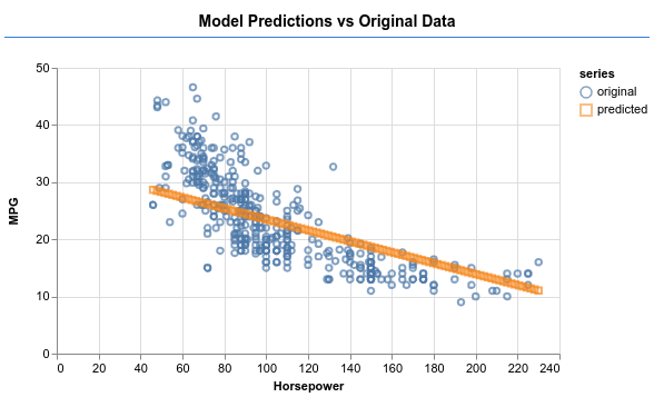
  tfvis.render.scatterplot(
    {name: 'Model Predictions vs Original Data'},
    {values: [originalPoints, predictedPoints], series: ['original', 'predicted']},
    {
      xLabel: 'Horsepower',
      yLabel: 'MPG',
      height: 300
    }
  );
}

This renders a scatterplot like so: